Contents
USAGE:
gsw_SA_CT_plot(SA,CT,p_ref,isopycs,title_string)
DESCRIPTION:
Produces a plot of Absolute Salinity - Conservative Temperature
profiles.  The diagram also plots the Conservative Temperature freezing
point for p = 0 dbar assuming the seawater is completely saturated with
dissolved air and user defined potential density contours.  This
function uses the computationally efficient 48-term expression for
density in terms of SA, CT and p (McDougall et al., 2011).
Note that the 48-term equation has been fitted in a restricted range of
parameter space, and is most accurate inside the "oceanographic funnel"
described in McDougall et al. (2011).  The GSW library function
"gsw_infunnel(SA,CT,p)" is avaialble to be used if one wants to test if
some of one's data lies outside this "funnel".
INPUT:
SA    =  Absolute Salinity                                     [ g/kg ]
CT    =  Conservative Temperature                             [ deg C ]
p     =  sea pressure                                          [ dbar ]
         ( i.e. absolute pressure - 10.1325 dbar )
Optional:
p_ref        = reference sea pressure for the isopycnals        [ dbar ]
               (i.e. absolute reference pressure - 10.1325 dbar)
               If it is not suppled a default of 0 dbar is used.
isopycs      = isopycnals, can be either an array of isopynals or the
               number of isopynals to appear on the plot.  If it is not
               supplied the programme defaults to 5 isopynals.
title_string = title text to appear at the top of the plot.
SA & CT need to have the same dimensions.
p_ref should be a scalar, (i.e. have dimensions 1x1).
isopycs can be either 1x1 or 1xN or Mx1
EXAMPLE:
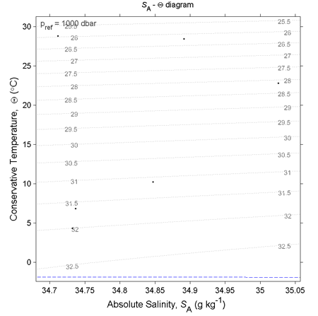
SA = [34.7118; 34.8915; 35.0256; 34.8472; 34.7366; 34.7324;]
CT = [28.8099; 28.4392; 22.7862; 10.2262;  6.8272;  4.3236;]
p =  [     10;      50;     125;     250;     600;    1000;]
p_ref = 1000
isopycs = [24:0.5:33];
gsw_SA_CT_plot(SA,CT,p_ref,isopycs,'\it{S}\rm_A - {\Theta} diagram')
AUTHOR:
Rich Pawlowicz                                 [ help@teos-10.org ]
Note. This function was extracted and adapted from Rich Pawlowicz's
 ocean toolbox.
Modified:
Paul Barker & Trevor McDougall
VERSION NUMBER:
3.01 (16th May, 2011).
REFERENCES:
IOC, SCOR and IAPSO, 2010: The international thermodynamic equation of
 seawater - 2010: Calculation and use of thermodynamic properties.
 Intergovernmental Oceanographic Commission, Manuals and Guides No. 56,
 UNESCO (English), 196 pp.  Available from the TEOS-10 web site.
McDougall T.J., P.M. Barker, R. Feistel and D.R. Jackett, 2011:  A
 computationally efficient 48-term expression for the density of
 seawater in terms of Conservative Temperature, and related properties
 of seawater.  To be submitted to Ocean Science Discussions.
This software is available from http://www.TEOS-10.org